Appendices
Appendix C
ColPali Appendix
Reproducibility Statement
For transparency, reproducibility and to foster future work, we release our training data, model checkpoints (adapters), entire codebase, and complete evaluation benchmark under MIT licenses as detailed in the main paper. We also host a public ViDoRe leaderboard to foster concurrent work in the space. The supplementary material further details training configurations for our models (also specified in HuggingFace model repositories), and dives into the process we used to generate synthetic data, how latency computations are performed, as well as provides further detailed evaluation results.
Acknowledgements
This work is partially supported by Illuin Technology, and by a grant from ANRT France. This work was performed using HPC resources from the CINES ADASTRA through Grant 2024-AD011015443 and from IDRIS with grant 2024-AD011015724R1. We extend our warm thanks to Jonathan Dong, Caio Corro, Victor Pellegrain and Ender Konukoglu for their valuable feedback on the paper.
Benchmark Datasets
Academic Datasets
DocVQA includes collected images from the UCSF Industry Documents Library. Questions and answers were manually annotated.
InfoVQA includes infographics collected from the Internet using the search query “infographics”. Questions and answers were manually annotated.
TAT-DQA is a large-scale Document VQA dataset that was constructed from publicly available real-world financial reports. It focuses on rich tabular and textual content requiring numerical reasoning. Questions and answers were manually annotated by human experts in finance.
arXivQA is a VQA dataset based on figures extracted from arXiv publications. The questions were generated synthetically using GPT-4 Vision.
TabFQuAD (Table French Question Answering Dataset) is designed to evaluate TableQA models in realistic industry settings. We create additional queries to augment the existing human-annotated ones using the same method described in Subsection C.3.2.
Practical Datasets
Methodology. Creating a relevant retrieval dataset close to real use cases is a major challenge as the dataset needs to be both sufficiently large for effective fine-tuning and sufficiently diverse to cover a broad range of modalities (full text, tables, charts, ...), domains (industry, healthcare, ...), and query-document interactions (extractive questions, open-ended questions, ...). Our approach to building this dataset involves several steps: (1) we use a web crawler to collect publicly available documents on various themes and sources, (2) we convert these PDFs into a series of images, one per page, and (3) we generate queries related to each image using a VLM.
Web-Crawler. We implemented a web crawler to efficiently collect large volumes of documents related to a given topic. The crawler is seeded with a user-defined query (e.g. “artificial intelligence") and then uses GPT-3.5 Turbo to brainstorm related topics and subtopics. This query augmentation strategy aims at both broadening and deepening the search. GPT-3.5 Turbo is further used to generate diverse search queries from each subtopic. This query set is then consumed by a pool of parallel workers whose job is to fetch the associated most relevant documents. We use SerpAPI along with a filetype filter (PDF documents only) to programmatically scrape Google Search rankings. Each file is hashed and stored in a Bloom filter shared among workers to avoid duplicate documents in the final corpus. Unique scraped files are downloaded, and inserted into a SQLite database along with additional metadata.
Datamix. Using the web crawler, we collected approximately 100 documents for each of the following four seeds: “energy", “government reports", “healthcare industry", and “artificial intelligence". These seeds were meticulously hand-picked to align with real-use cases for retrieval models and visually rich pages. We also removed all documents containing any private information.
Query Generation. To increase the efficiency of our query generation scheme and to limit API calls, we generate at most 3 questions per image. From all the documents collected, we randomly sample 10,000 images per theme and call Claude-3 Sonnet with the following prompt:
Human Validation. We manually validate every single synthetically created query in ViDoRe to ensure quality, query relevance, and consistency with the benchmark objective of evaluating retrieval in practical industrial settings. During this step, we randomly assign document-pair queries to 4 volunteer annotators and instruct them to filter out queries that do not fit the above-listed criteria. We also instruct annotators to flag any documents they deem to contain PII information or content not suited for an academic benchmark. No flag was raised during the entirety of the process, validating our prior PDF collection strategy. 100 queries per topic are collected in this manner. Annotators are colleagues and collaborators of the authors who volunteered to help. Each annotator spent approximately 3 hours filtering the larger query set down to 100 high-quality queries per topic.
Training Dataset
The statistics of the train set are given in the following table. The creation of the train set follows the same methodology as in Subsection C.3.2. We made sure that a PDF document cannot have pages in both the training set and the test set to prevent data leakage and that there are no duplicate documents in each split.
| Dataset Split | Split Size | Language | Domain |
| DocVQA | 39,463 | English | Scanned documents from UCSF Industry |
| InfoVQA | 10,074 | English | Infographics scraped from the web |
| TATDQA | 13,251 | English | High-quality financial reports |
| arXivQA | 10,000 | English | Scientific Scientific Figures from arXiv |
| Scraped PDFs | 45,940 | English | Varied PDFs from 3885 distinct URL domains |
| TOTAL | 118,695 | English-only | Mixed |
Implementation details
Codebase
The codebase is written in PyTorch and leverages HuggingFace tooling for model implementations and trainers.
Hyperparameters
Hyperparameters are tuned on a validation split composed of of the training dataset. We find bi-encoder methods to be more sensible to learning rate variations than late interaction-based models and achieve the best performance for all models with a learning rate of . We experiment with LoRA rank and values and do not notice particular improvements past . Per-device batch sizes are kept small due to long sequence lengths that complicate scaling past . We simulate larger batch sizes with multi-GPU training and train with a total batch size with no accumulation, for 1 epoch on our training set.
Embedding size
Minimizing storage footprint can be essential to industrial retrieval systems if databases contain millions of documents. With this criterion in view, we have compared the embedding sizes of the models in our study. As shown in Table 2, ColPali’s embedding size is an order of magnitude larger than BM25 and two orders of magnitude larger than BGE-M3. However, in practical scenarios, pooling multi-vector embeddings by centroid cluster, or quantizing embeddings to binary representations can reduce storage costs by two orders of magnitude with minimal performance hits, and make storage costs competitive with other systems.
| Model | Embedding size (KB) |
| BGE-M3 | 8.60 |
| BM25 (dense emb.) | 3.00 |
| BM25 (sparse emb.) | 1.56 ± 0.51 |
| ColPali (float16) | 257.5 |
Latency computations
To ensure comparison fairness, the latencies of the different retrieval systems shown in Figure 2 are measured on the same g2-standard-8 GCP VM with an NVIDIA L4 GPU. Document pages are embedded using the highest settings of Unstructured with captioning (see Subsection 3.3.2). SigLIP and ColPali are both loaded with bfloat16 parameter dtypes. The reported times in Table 3 are the average per-page latencies for each indexing operation on 1000 randomly chosen documents across all splits of the ViDoRe benchmark test set. A batch size of was used for the BGE-M3 model used with Unstructured, and a batch size of was used for SigLIP and ColPali.
| Indexing operation | Latency (s) | ||
| Unstructured | SigLIP | ColPali | |
| Layout detection | 0.81 | NA | NA |
| OCR | 2.67 | NA | NA |
| Captioning | 3.71 | NA | NA |
| Page encoding | 0.03 | 0.12 | 0.39 |
| Total | 7.22 | 0.12 | 0.39 |
Captioning
Examples of captions generated for visually rich document chunks with Claude-3 Sonnet are shown in Figure 2 and Figure 1. The prompt used for generating the description is the following:
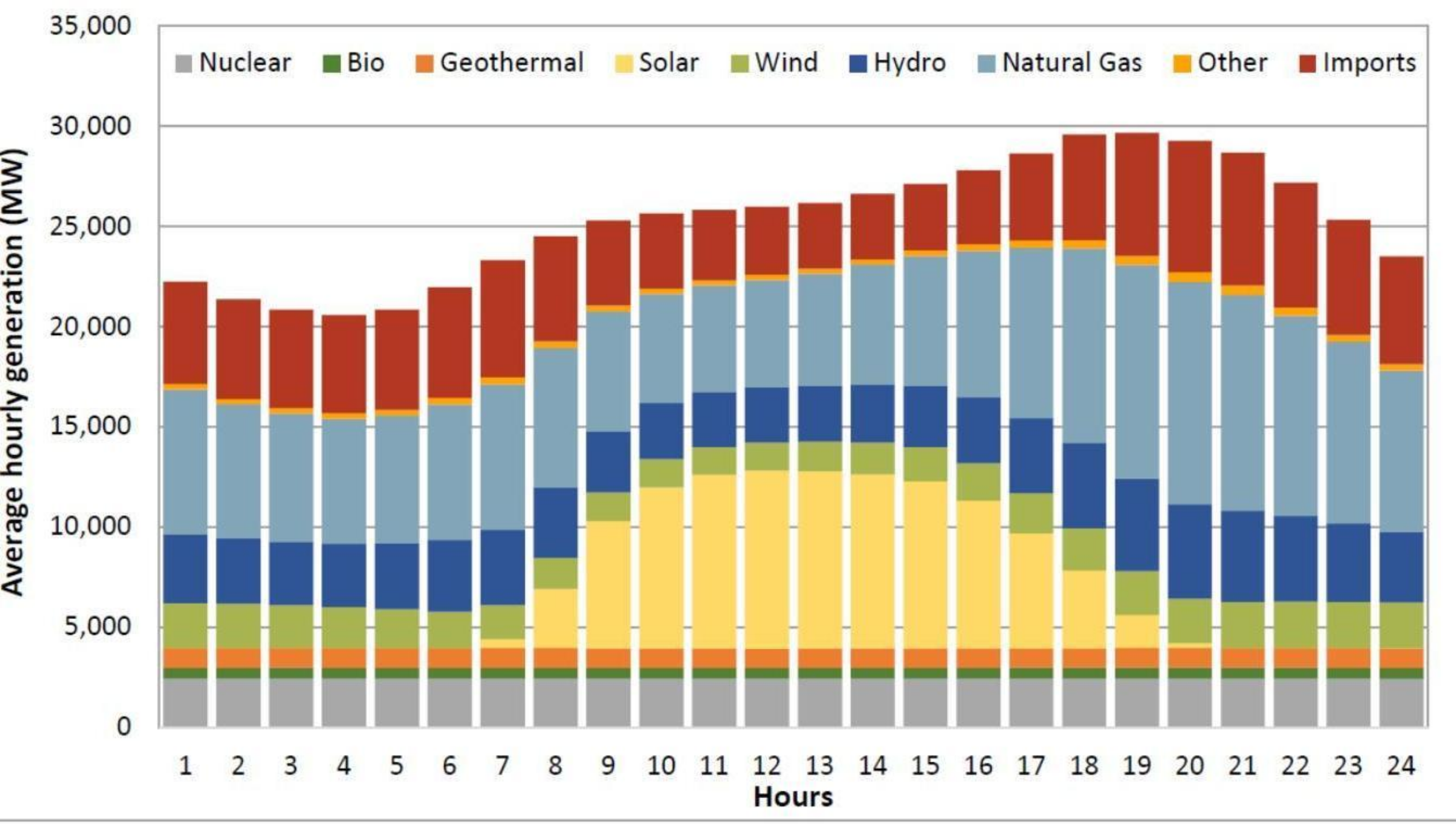
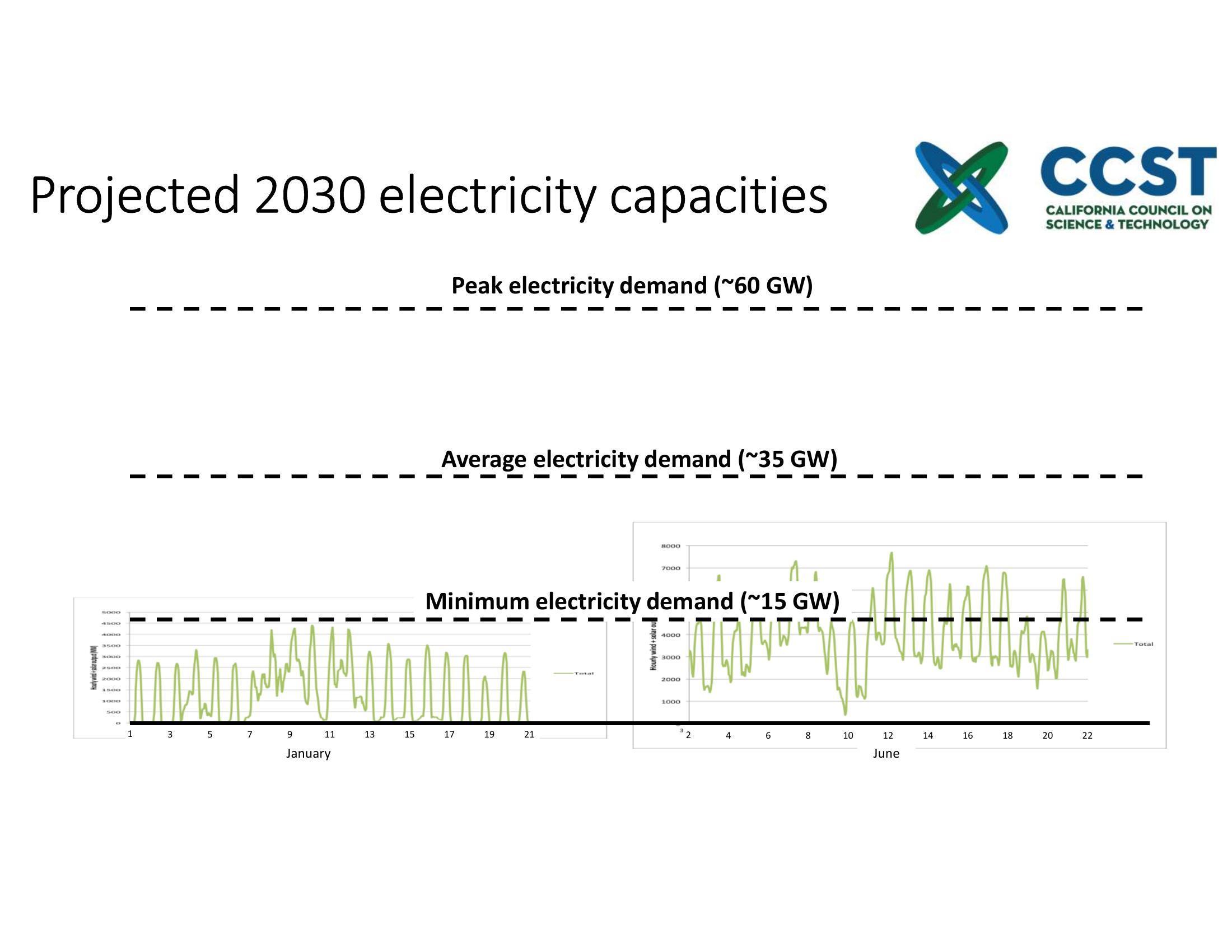
Caption: The image depicts the hourly energy generation profile, illustrating the contributions of various energy sources over 24 hours. The data is presented as a stacked bar chart, with the x-axis representing the hours of the day from 1 to 2, and the y-axis showing the average hourly generation in MW. The bars are segmented into different colors, each representing a distinct energy source: nuclear, bio, geothermal, solar, wind, hydro, natural gas, and other imports. The chart provides insights into the temporal variations in energy generation across different sources, highlighting the interplay between baseload and intermittent sources throughout the day.
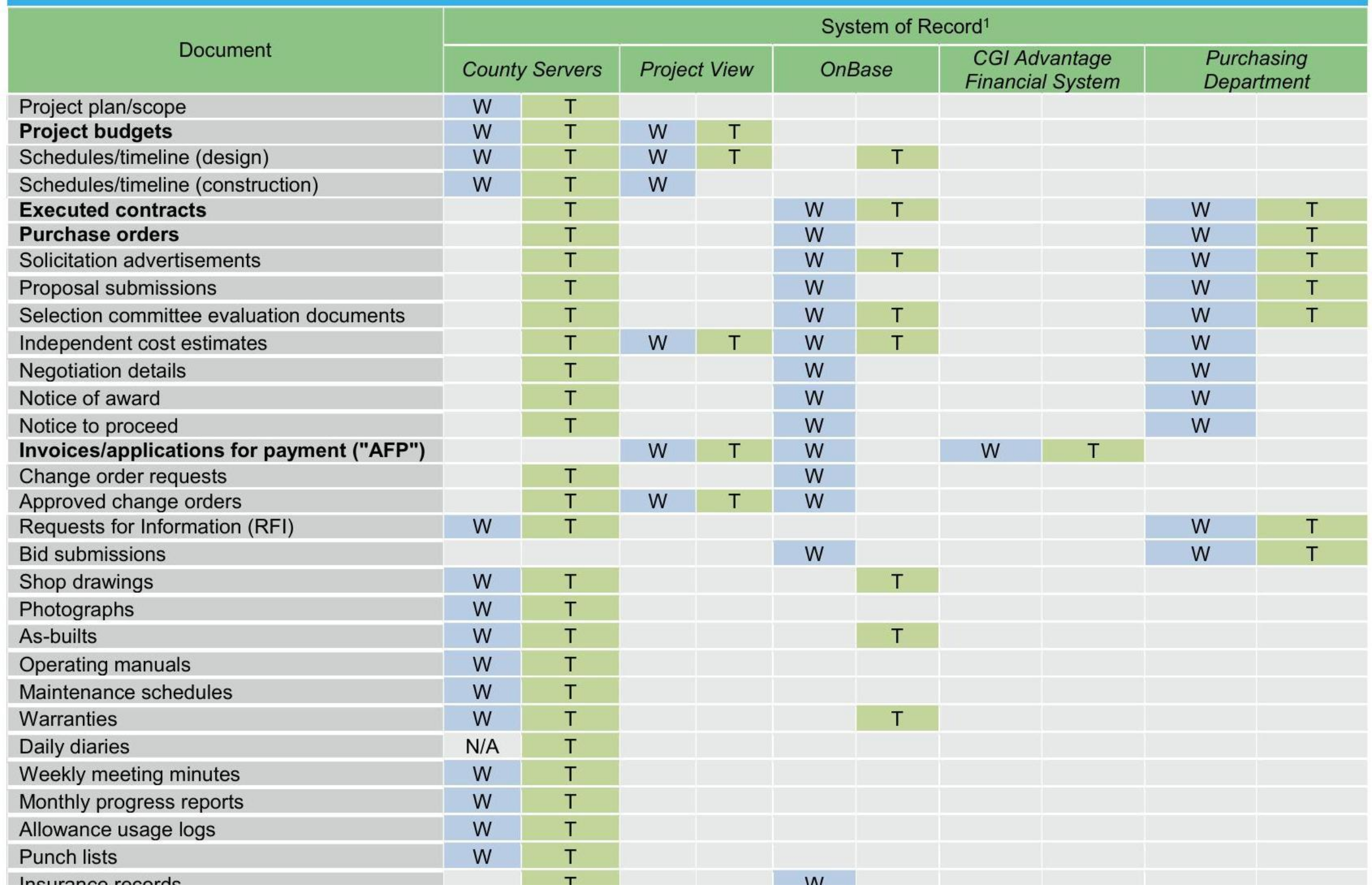
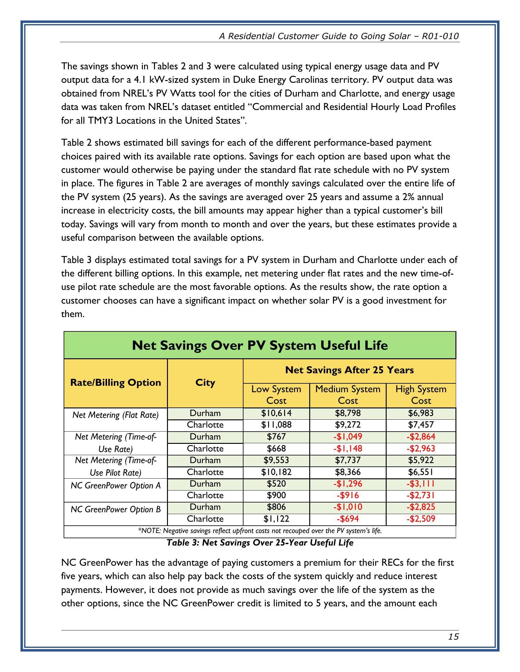
Caption: The image shows a table titled “System of Record" which outlines the different types of documents or records maintained across various systems or departments within an organization related to project management and construction. The rows list documents like project plans, budgets, schedules, contracts, purchase orders, invoices, change requests, bid submissions, drawings, manuals, meeting minutes, and reports. The columns indicate the system or department responsible for maintaining each record, such as County Servers, Project View, OnBase, CGI Advantage Financial System, and Purchasing Department. The table uses "W" and "T" markers to denote which system or department serves as the primary source (writer) or storage location (trailer) for each type of document.
Additional results
Other Metrics
| ArxivQ | DocQ | InfoQ | TabF | TATQ | Shift | AI | Energy | Gov. | Health. | Avg. | |
Unstructured text-only | |||||||||||
| BM25 | - | 26.6 | - | - | 34.6 | 45.0 | 86.0 | 70.0 | 68.0 | 74.0 | - |
| BGE-M3 | - | 22.83.8 | - | - | 26.18.5 | 51.06.0 | 81.05.0 | 72.02.0 | 67.01.0 | 77.03.0 | - |
Unstructured i͡ny+ OCR | |||||||||||
| BM25 | 26.7 | 28.9 | 54.0 | 30.4 | 50.0 | 52.0 | 86.0 | 77.0 | 74.0 | 80.0 | 55.9 |
| BGE-M3 | 28.11.4 | 22.96.0 | 53.80.2 | 55.725.3 | 38.611.4 | 56.04.0 | 82.04.0 | 79.02.0 | 76.02.0 | 83.03.0 | 57.51.6 |
Unstructured + Captioning | |||||||||||
| BM25 | 35.5 | 30.2 | 61.5 | 24.3 | 49.0 | 47.0 | 79.0 | 76.0 | 75.0 | 81.0 | 55.9 |
| BGE-M3 | 29.36.2 | 26.04.2 | 62.1 0.6 | 58.634.3 | 30.618.4 | 55.08.0 | 80.01.0 | 78.02.0 | 69.06.0 | 83.02.0 | 57.21.3 |
| Contrastive VLMs | |||||||||||
| Jina-CLIP | 19.4 | 7.3 | 26.7 | 12.5 | 1.6 | 2.0 | 11.0 | 13.0 | 15.0 | 17.0 | 12.6 |
| Nomic-vision | 10.4 | 6.7 | 22.1 | 9.6 | 1.6 | 0.0 | 9.0 | 9.0 | 7.0 | 13.0 | 8.8 |
| SigLIP (Vanilla) | 34.2 | 21.3 | 51.8 | 46.1 | 17.9 | 13.0 | 50.0 | 51.0 | 47.0 | 65.0 | 39.7 |
| Ours | |||||||||||
| SigLIP (Vanilla) | 34.2 | 21.3 | 51.8 | 46.1 | 17.9 | 13.0 | 50.0 | 51.0 | 47.0 | 65.0 | 39.7 |
| BiSigLIP (+fine-tuning) | 49.215.0 | 23.82.5 | 59.07.2 | 52.16.0 | 20.72.8 | 16.03.0 | 62.012.0 | 61.010.0 | 55.08.0 | 72.07.0 | 47.17.4 |
| BiPali (+LLM) | 46.4-2.8 | 20.0-3.8 | 54.6-4.4 | 63.211.1 | 20.4-0.4 | 34.018.0 | 59.0-3.0 | 45.0-16.0 | 57.02.0 | 56.0-16.0 | 45.6-1.5 |
| ColPali (+Late Inter.) | 72.426.0 | 45.625.6 | 74.620.0 | 75.412.1 | 53.132.7 | 55.021.0 | 93.034.0 | 85.040.0 | 85.028.0 | 88.032.0 | 72.727.1 |
Model Variants
| ArxivQ | DocQ | InfoQ | TabF | TATQ | Shift | AI | Energy | Gov. | Health. | Avg. | |
| ColSigLIP (PaliGemma) | 3.1 | 3.0 | 5.1 | 6.2 | 2.5 | 1.0 | 3.4 | 3.4 | 2.3 | 2.2 | 3.2 |
| BiSigLIP (PaliGemma) | 18.5 | 14.6 | 33.4 | 39.5 | 16.1 | 5.2 | 27.6 | 32.6 | 36.6 | 35.7 | 26.0 |
| ColSigLIP (Original) | 2.6 | 2.2 | 2.3 | 5.7 | 1.8 | 1.0 | 2.6 | 4.1 | 1.4 | 1.5 | 2.5 |
| ColPali (No Q.A. Tokens) | 80.4 | 53.2 | 82.4 | 77.4 | 65.7 | 63.4 | 97.0 | 89.9 | 93.6 | 92.4 | 79.6 |
| ColPali (Docmatix) | 71.3 | 48.0 | 80.0 | 83.9 | 59.1 | 73.8 | 95.7 | 93.8 | 92.5 | 93.1 | 79.1 |
| ColPali (224) | 71.0 | 37.4 | 62.3 | 65.7 | 28.6 | 20.4 | 65.7 | 66.8 | 73.9 | 73.0 | 56.5 |
| ColPali (Vision Trained) | 78.8 | 53.9 | 81.3 | 81.7 | 64.4 | 70.6 | 95.3 | 91.7 | 93.5 | 94.7 | 80.6 |
| ColPali (No Pairwise) | 79.0 | 53.0 | 82.1 | 85.3 | 63.2 | 66.2 | 94.9 | 88.9 | 92.7 | 92.1 | 79.7 |
| ColPali (+TabFQuAD training) | 77.6 | 54.7 | 82.6 | 86.5 | 65.4 | 73.9 | 94.8 | 92.4 | 94.2 | 94.8 | 81.7 |
| ColIdefics2 (64) | 73.6 | 48.0 | 82.4 | 81.6 | 63.0 | 57.2 | 95.5 | 86.9 | 86.6 | 91.2 | 76.6 |
| ColQwen2 (768) | 86.4 | 56.2 | 89.8 | 88.7 | 75.2 | 85.7 | 98.8 | 94.8 | 93.6 | 97.3 | 86.6 |
| ColPali (Reference: 448) | 79.1 | 54.4 | 81.8 | 83.9 | 65.8 | 73.2 | 96.2 | 91.0 | 92.7 | 94.4 | 81.3 |
More similarity maps
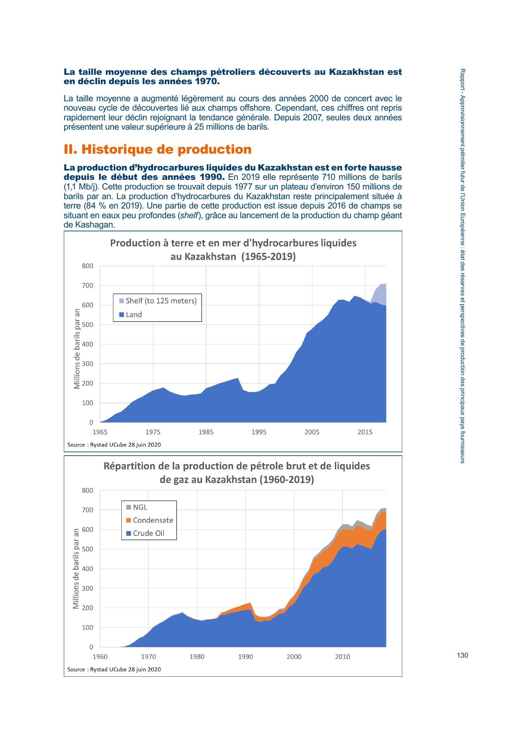
In Figure 3, ColPali assigns a high similarity to all patches with the word “Kazakhstan" when given the token <\_Kazakhstan>. Moreover, our model seems to exhibit world knowledge capabilities as the patch around the word "Kashagan"—an offshore oil field in Kazakhstan—also shows a high similarity score.
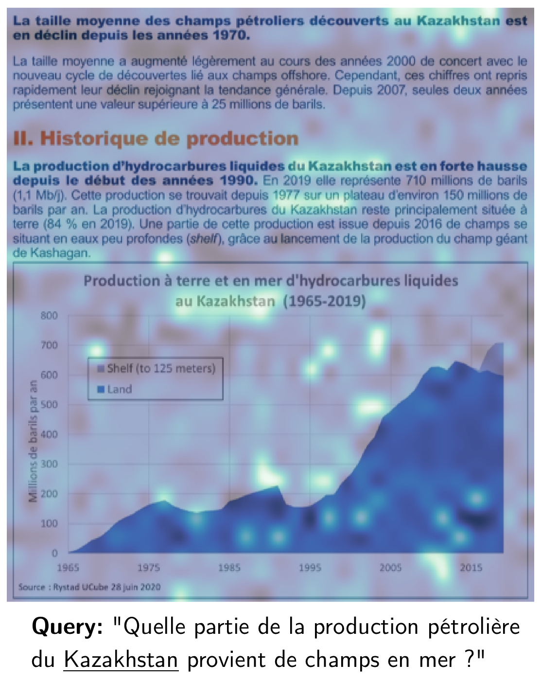
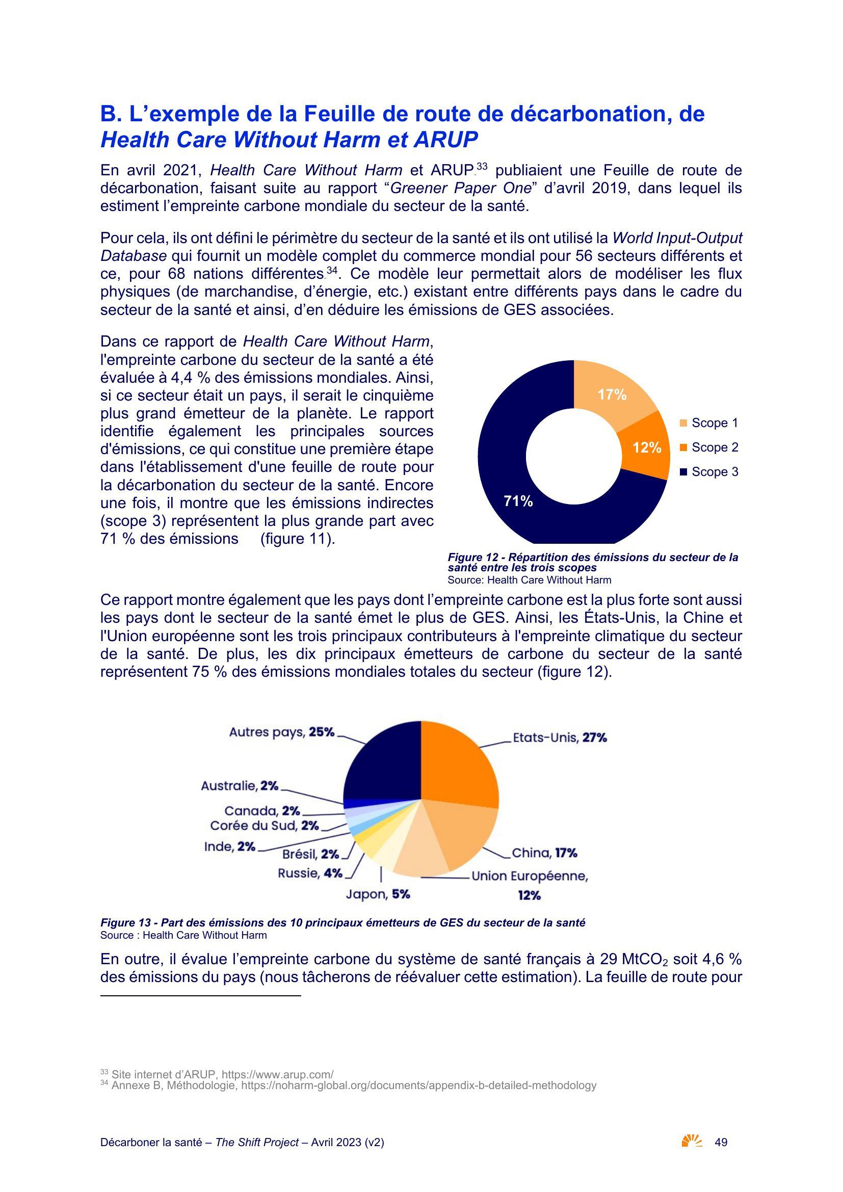
It is also interesting to highlight that both this similarity map and the one displayed in Figure 4 showcase a few white patches with high similarity scores. This behavior might first seem surprising as the white patches should not carry a meaningful signal from the original images. We believe the vectors associated with these patches share a similar role with the ViT registers , i.e. these patches were repurposed for internal computations and stored the global information from the whole image.
Model glossary
SigLIP
SigLIP (Sigmoid Loss for Language Image Pre-Training) builds upon CLIP (Contrastive Language-Image Pretraining)—a foundational model that aligns images and text by maximizing the similarity between correct image-text pairs while minimizing it for incorrect ones, leveraging a contrastive loss . Unlike CLIP , which applies the softmax function to the logits, SigLIP uses the sigmoid activation function. This innovation eliminates the need for a global view of all pairwise similarities between images and texts within a batch, enabling more flexible batch size scaling (up to 1M items per batch, with an effective optimal batch size of 32k). This approach allows SigLIP to achieve state-of-the-art performance in zero-shot image classification tasks.
PaliGemma
PaliGemma is a 3B-parameter vision-language model. It integrates the SigLIP vision encoder with a Gemma-2B language decoder, connected via a multimodal linear projection layer . The model processes images by segmenting them into a fixed number of Vision Transformer tokens, which are prepended to an optional text prompt.
A distinguishing feature of PaliGemma is its operation as a Prefix-Language Model (Prefix-LM). This design ensures full attention between image tokens and the user-provided input (prefix) while generating outputs auto-regressively (suffix). This architecture allows image tokens to access the task-specific query during processing, facilitating more effective task-dependent reasoning.
PaliGemma was trained in four stages: unimodal pretraining with existing components, extended multimodal pretraining, short high-resolution pretraining, and task-specific fine-tuning.
ColBERT
ColBERT (Contextualized Late Interaction over BERT) is a retrieval model designed to balance speed and effectiveness in information retrieval tasks . Traditional retrieval models are typically categorized based on their type of interaction: either processing queries and documents independently for efficiency (bi-encoders) or jointly to capture rich contextual relationships (cross-encoders). ColBERT combines the advantages of both approaches through a novel late interaction mechanism.
Queries and documents are encoded separately using BERT, enabling offline pre-computation of document representations for scalability. Instead of pooling embeddings into a single vector, ColBERT retains token-level embeddings and employs a MaxSim operator to compute fine-grained similarity scores. For each query token, the model determines the maximum similarity with document tokens, summing these scores to compute relevance.
This architecture preserves the contextual richness of deep language models while significantly improving computational efficiency. By delaying the interaction step, ColBERT supports vector similarity indexing, facilitating end-to-end retrieval from large collections without prohibitive costs. Empirical evaluations on passage search datasets demonstrate that ColBERT achieves competitive effectiveness compared to existing BERT-based models , while executing queries orders of magnitude faster and with drastically reduced computational requirements.
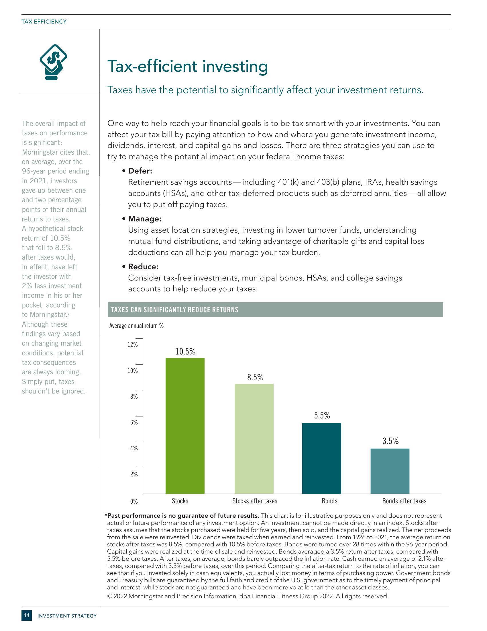
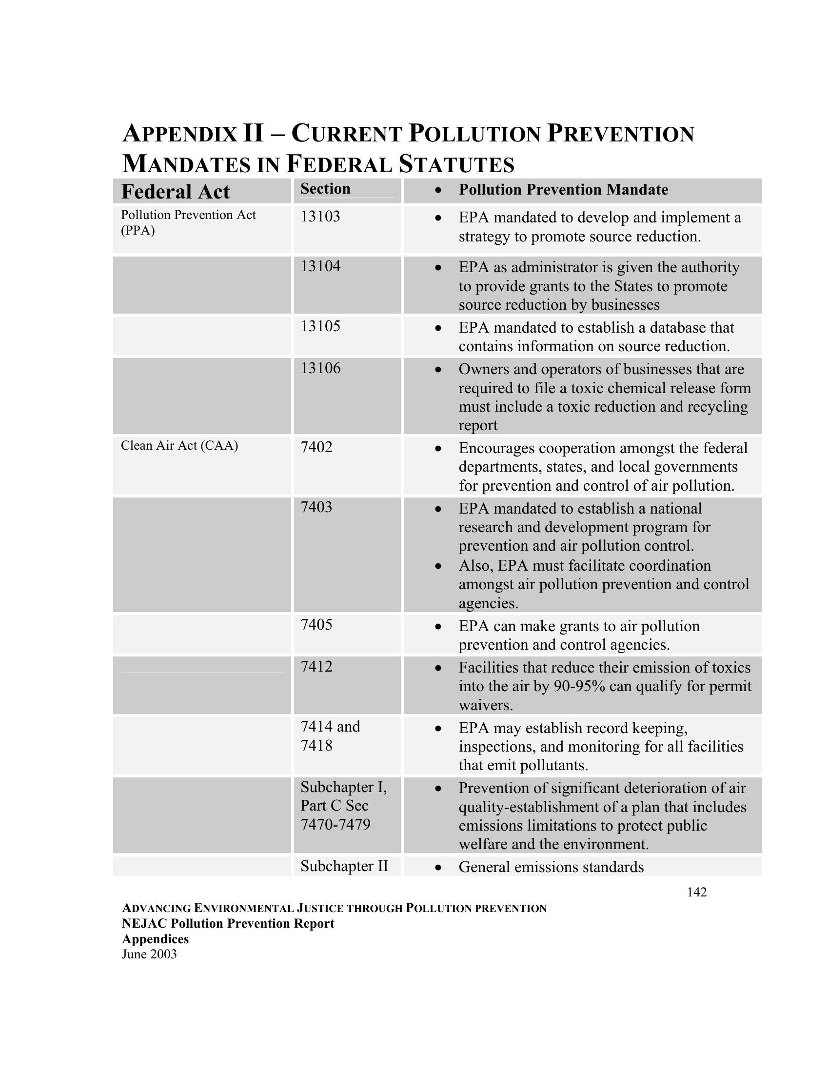
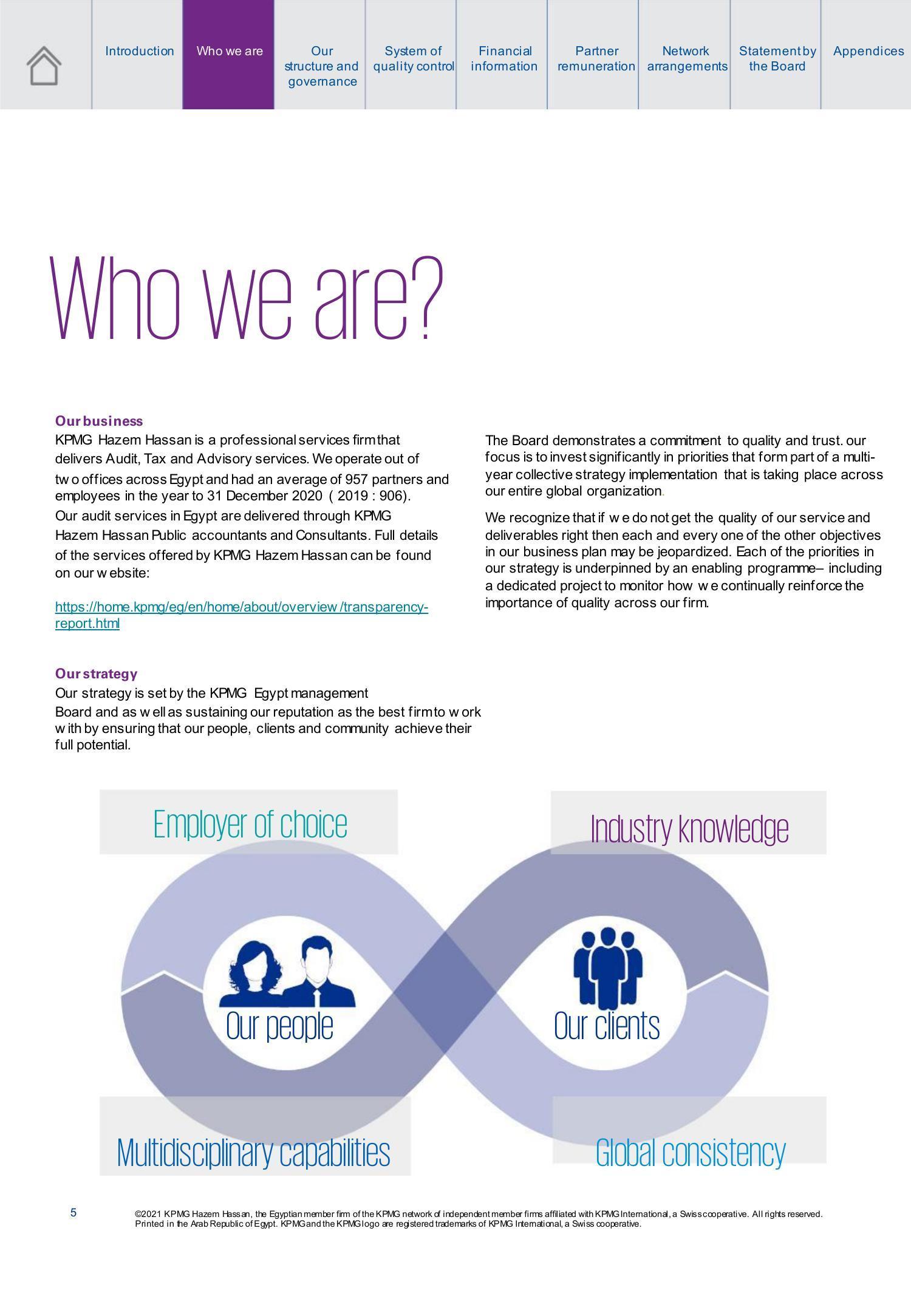
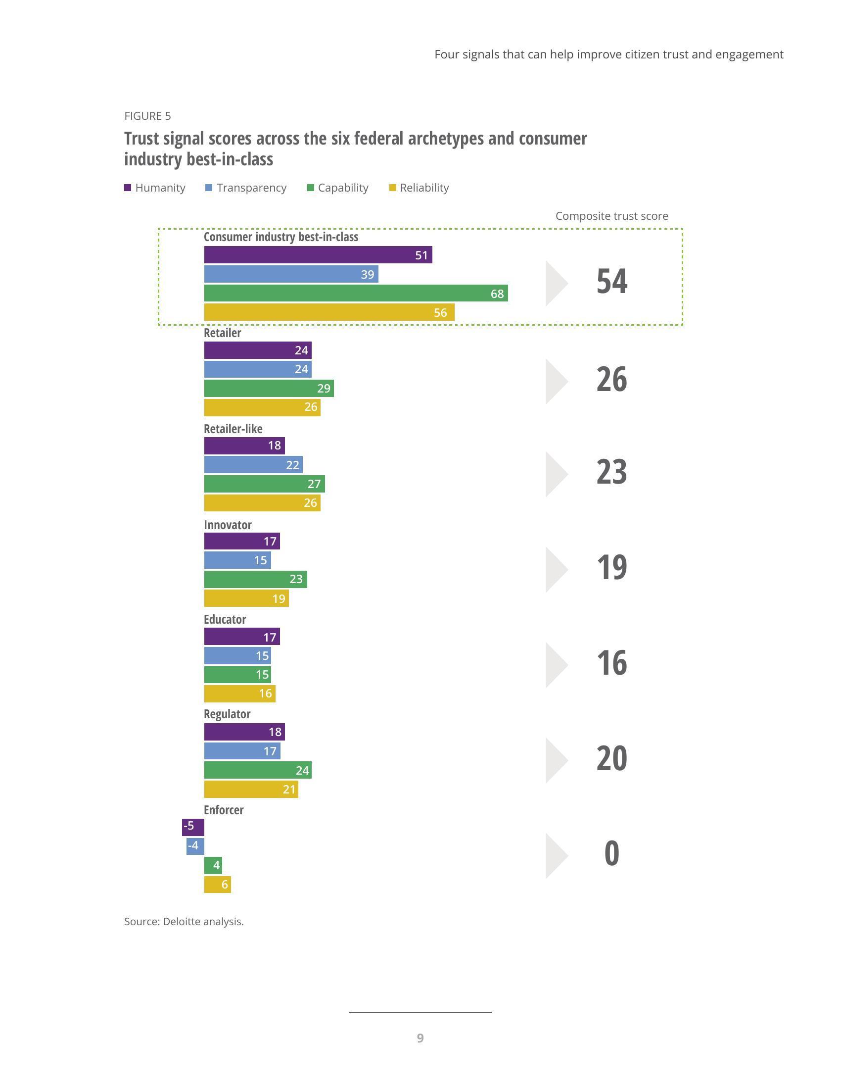
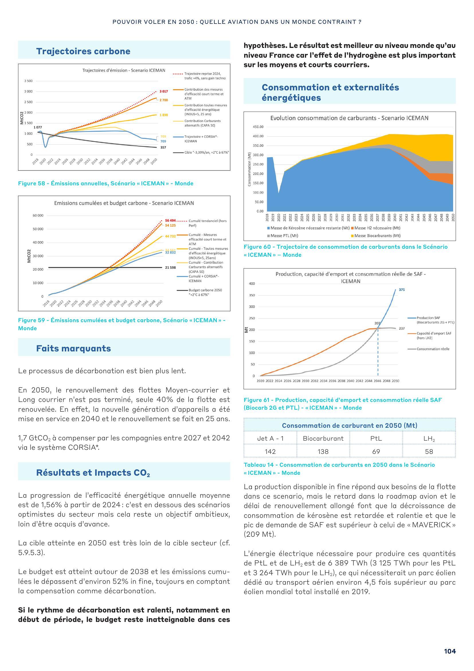
Examples from the ViDoRe benchmark
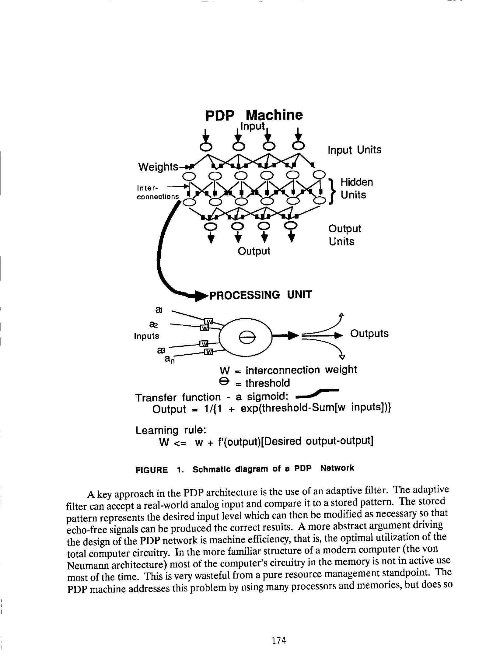
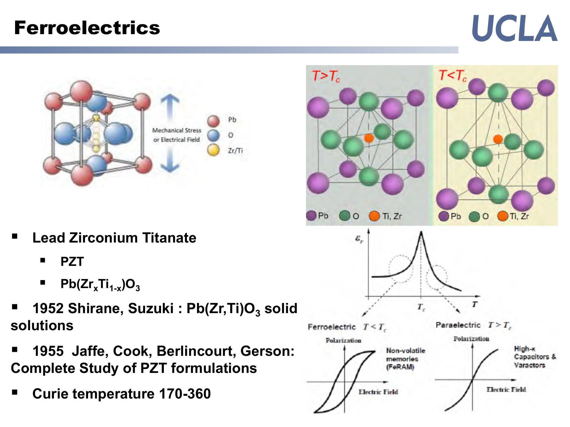
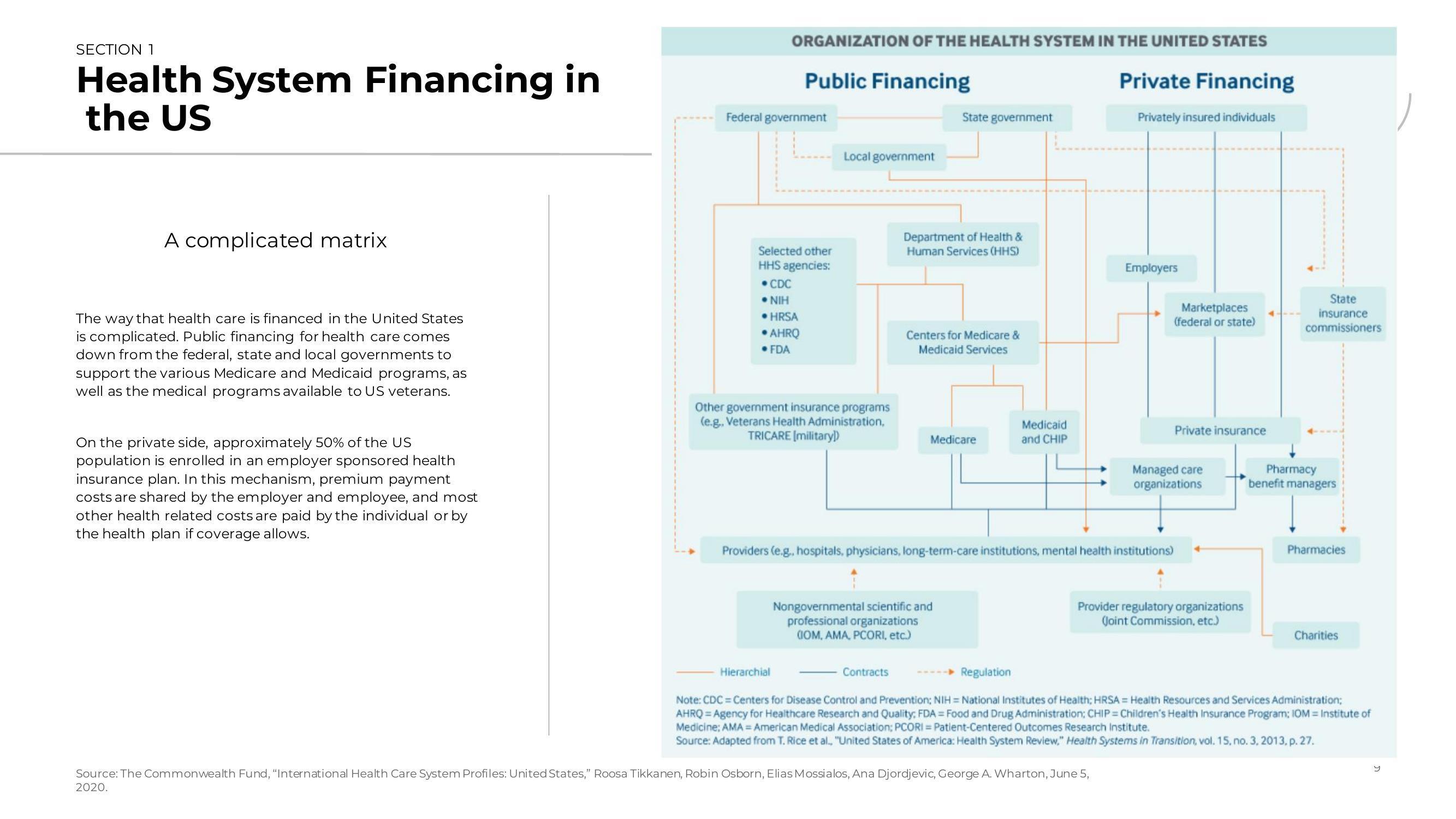
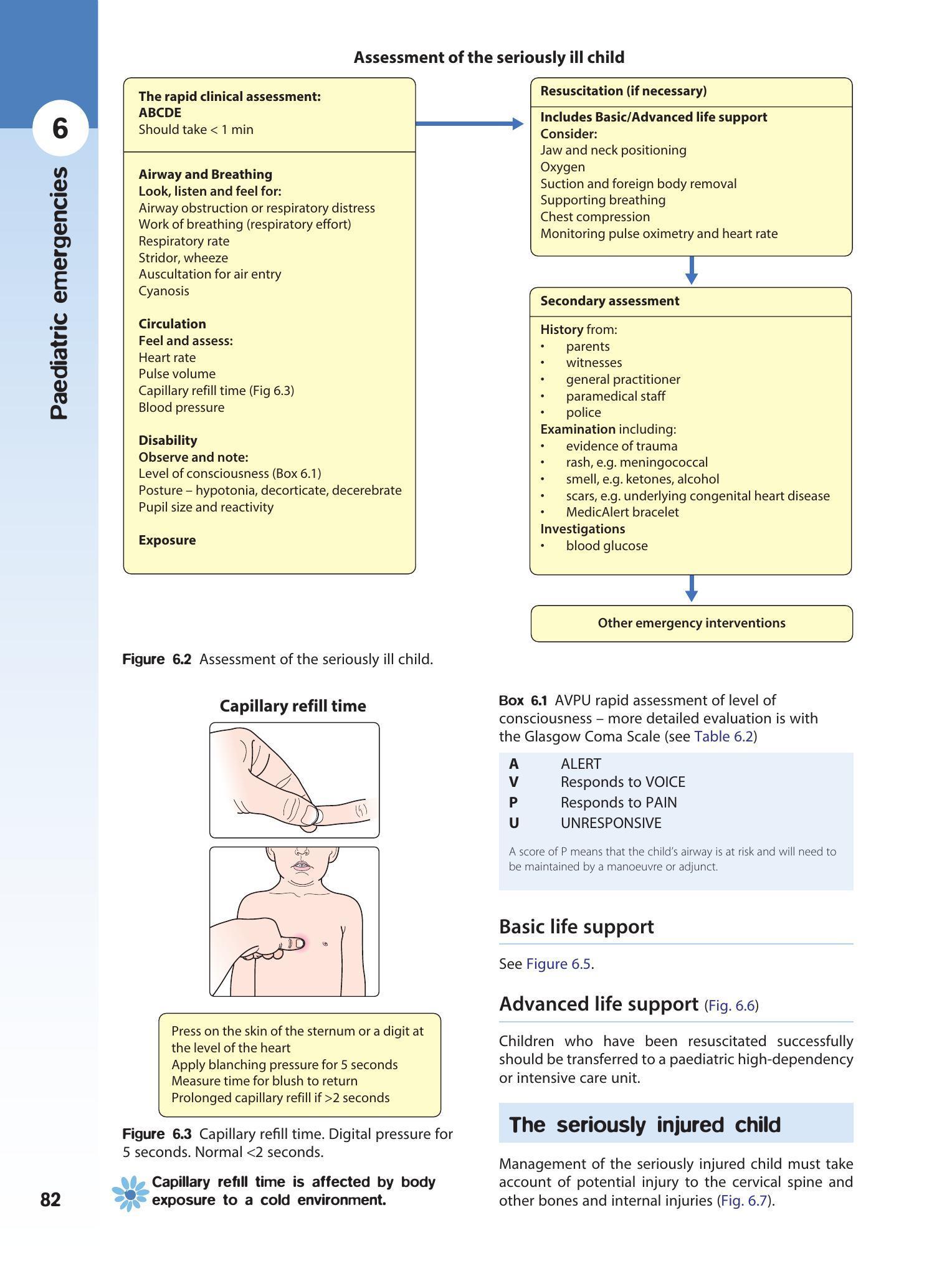
References
- Minesh Mathew, Dimosthenis Karatzas, C. V. Jawahar (2020). DocVQA: A Dataset for VQA on Document Images. Source ↗
- Minesh Mathew, Viraj Bagal, Rubèn Pérez Tito, Dimosthenis Karatzas, Ernest Valveny, C. V Jawahar (2021). InfographicVQA. arXiv. Source ↗
- Fengbin Zhu, Wenqiang Lei, Fuli Feng, Chao Wang, Haozhou Zhang, Tat-Seng Chua (2022). Towards Complex Document Understanding By Discrete Reasoning. Source ↗
- Lei Li, Yuqi Wang, Runxin Xu, Peiyi Wang, Xiachong Feng, Lingpeng Kong, Qi Liu (2024). Multimodal ArXiv: A Dataset for Improving Scientific Comprehension of Large Vision-Language Models.
- Burton H. Bloom (1970). Space/time trade-offs in hash coding with allowable errors. Source ↗
- Keshav Santhanam, Omar Khattab, Christopher Potts, Matei Zaharia (2022). PLAID: An Efficient Engine for Late Interaction Retrieval. arXiv. Source ↗
- Timothée Darcet, Maxime Oquab, Julien Mairal, Piotr Bojanowski (2023). Vision Transformers Need Registers. Source ↗
- Xiaohua Zhai, Basil Mustafa, Alexander Kolesnikov, Lucas Beyer (2023). Sigmoid Loss for Language Image Pre-Training. Source ↗
- Alec Radford, Jong Wook Kim, Chris Hallacy, Aditya Ramesh, Gabriel Goh, Sandhini Agarwal, Girish Sastry, Amanda Askell, Pamela Mishkin, Jack Clark, Gretchen Krueger, Ilya Sutskever (2021). Learning Transferable Visual Models From Natural Language Supervision. Source ↗
- Lucas Beyer*, Andreas Steiner*, André Susano Pinto*, Alexander Kolesnikov*, Xiao Wang*, Xiaohua Zhai*, Daniel Salz, Maxim Neumann, Ibrahim Alabdulmohsin, Michael Tschannen, Jeremiah Harmsen, Daniel Keysers, Neil Houlsby, Xi Chen, Emanuele Bugliarello, Thomas Unterthiner, Keran Rong, Matthias Minderer, Ioana Bica, Ivana Balazevic, Joan Puigcerver, Julian Eisenschlos, Manoj Kumar, Matko Bošnjak, Matthias Bauer, Fangyu Liu, Adam Grycner, Alexey Gritsenko, Paul Voigtlaender, Pinelopi Papalampidi, Olivier Henaff, Skanda Koppula, Xi Xiong, Radu Soricut, Model release contributors, general support, Tris Warkentin, Kat Black, Luiz Gustavo Martins, Glenn Cameron, Raj Gundluru, Manvinder Singh, Meg Risdal, Nilay Chauhan, Nate Keating, Nesh Devanathan, Elisa Bandy, Joe Fernandez, Antonia Paterson, Jenny Brennan, Tom Eccles, Pankil Botadra, Ben Bariach, Lav Rai, Minwoo Park, Dustin Luong, Daniel Vlasic, Bo Wu, Wenming Ye, Divyashree Sreepathihalli, Kiranbir Sodhia, Alek Andreev, Armand Joulin, Surya Bhupatiraju, Minh Giang, Joelle Barral, Zoubin Ghahramani (2024). PaliGemma. Kaggle. Source ↗
- Alexey Dosovitskiy, Lucas Beyer, Alexander Kolesnikov, Dirk Weissenborn, Xiaohua Zhai, Thomas Unterthiner, Mostafa Dehghani, Matthias Minderer, Georg Heigold, Sylvain Gelly, Jakob Uszkoreit, Neil Houlsby (2020). An Image is Worth 16x16 Words: Transformers for Image Recognition at Scale. Source ↗
- Omar Khattab, Matei Zaharia (2020). ColBERT: Efficient and Effective Passage Search via Contextualized Late Interaction over BERT. Proceedings of the 43rd International ACM SIGIR Conference on Research and Development in Information Retrieval. Source ↗
- Jacob Devlin, Ming-Wei Chang, Kenton Lee, Kristina Toutanova (2019). BERT: Pre-training of Deep Bidirectional Transformers for Language Understanding. Proceedings of the 2019 Conference of the North American Chapter of the Association for Computational Linguistics: Human Language Technologies, Volume 1 (Long and Short Papers). Source ↗